December 11, 2016 / by Vikram Sachdeva / In news

Final Report

Here is our code.
Here is our powerpoint.
Here are examples of our transformations.

TOOLS USED:

MFCC: Mel Frequency Cepstrum Coefficients (MFCCs) are a common way of representing spoken word signals such in DSP. The inspiration for this feature vector is taken from how the human ear processes sound. The MFCC vector of a signal segment is generated as follows:
1. Take the Fourier Transform of a windowed signal.
2. Calculate the power spectrum of the Fourier Transform.
3. Apply a filter that takes the power spectrum and defines it with twenty six bins. Each bin describes the power of a certain range of frequencies, and there can be overlap between bins. This process is described as passing the power spectrum through a mel filter. These bins apply a filter that separates the spectrum into 26 bins, 13 in the negative frequency section of the Fourier Transform and 13 in the positive section. Because the signal we transformed is real-value, the negative frequency components of the Fourier Transform are equal to the complex conjugate of the corresponding positive frequency components, so we can actually define only 13 bins. These bins are spaced exponentially, with higher frequency bins covering a larger range of frequencies. This mimics the way that the human ear processes sound.
4. Take the log of each of these binned values. This approximates the way that the human ear processes loudness, which is on a logarithmic scale, like the decibel.
5. Take the Discrete Cosine Transform of the 26 power banks. This is required to make certain that the signal is real valued.

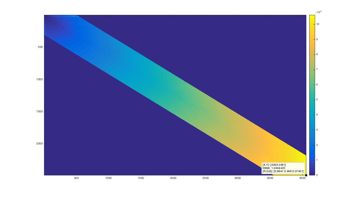
Dynamic Time Warping: Dynamic Time Warping (DTW) is an algorithm that calculates similarities between two discrete time signals that vary in speed and length. For our project, this was particularly valuable due to the fact that words can be spoken at different rates. This algorithm allowed us to build one concise classifier for a speaker on a training sentence, and then allowed us to generalize it. This algorithm generates an n by m matrix, where n is the length of one signal, and m is the length of our other signal. Each indices of the matrix denotes euclidian distance between the two signals at a certain point in time. Then we find the least weighted path from (n, m) to (1,1). This least weighted path describes the optimal mapping from timepoints of one vector to timepoints of the other vector. The following figure is a plot of the cumulative weight map that is created as an intermediate step in DTW. Only values reasonably close to the diagonal are calculated because it is assumed that the signals will not diverge too greatly.

K-Nearest Neighbors for Classification: In order to classify the phonemes in our samples, we used K-Nearest Neighbors (KNN) classification. This classification algorithm inputs an unlabeled data vector and a set of labeled vectors. The Euclidean distance from each labeled vector to the unlabeled vector (i.e., the norm of the difference vector between the two) is calculated, and for some number K, the K labeled vectors with the smallest distance are taken. A “majority vote” is taken, where the most common label in this set of K labels is assigned to the unlabeled vector. In the case of a tie, the label of the closest vector among the tied vectors is used.

METHODS AND PROCEDURE:

Our project required an effective way to quantify a given speech signal’s phonemes. The problem we encountered was that spoken speech can be imprecise, unpredictable, and variable and these disfluencies carry into the time domain. Rather than investigating the signal in the time domain, we chose use to use MFCCs as our feature vector. While a few linguistic papers do investigate phoneme classification in the time domain, we found academic literature to heavily favor analysis through MFCCs and thereby chose this route.

Feature vectors are defined as a vector containing information describing an object’s key characteristics. This is similar to non-redundant columns that span a matrix’s subspace, or a RGB vector describing a pixel’s color in an image. After implementing a toolbox that computed MFCCs for us, we wanted to use K-nearest Neighbors as our phoneme classification scheme. We considered two other classification methods: Bayesian and Support Vector Machine. To create a Bayesian model, you must obtain reasonable estimates for the probability of a given feature vector, the probability of a given phoneme, and the probability of a feature vector given it is of a certain type of phoneme. We did not have reliable ways to generate these probabilities, so we decided against a Bayesian model. A Support Vector Machine would divide up the 13-dimensional feature space into regions, with each region corresponding to one phoneme; any vector that lies inside a certain space is classified as that phoneme. We found this to be unsuccessful, which we hypothesized was due to variations and overlap in MFCCs of different phonemes. K-Nearest Neighbors actually worked very well for us.

To begin KNN classification, Paul spoke a sentence that contains all of the phonemes of the English language, and then recited each of the 44 phonemes of in the English language 5 times. The recitation of the phonemes will be hereby referred to as our training data. After using Audacity to split speech into the separate phonemes, we implemented a toolbox that computed the the full 13 dimensional space of MFCCs of the training data.

As a time-saving technique, instead of splicing out each individual phoneme, we split the audio signal into segments containing all five phonemes of the same type. We then calculated the energy in the signal over each 10ms interval, by summing the squares of the sample values. We took the 15 highest amplitude intervals to be the best, in terms of SNR, and used them as our dictionary elements for each phoneme. This way we had an equal amount of elements for each label in our dictionary, so we did not have any bias in our classification.

Considering the 13 dimensional space of MFCCs, our KNN classifier gave us an error rate of 21.0% for phoneme classification and 1.48% for vowel classification, using leave one out cross validation to assert accuracy. Phoneme classification is defined as binning all of the phonemes in the spoken sentence to every phoneme in our data set, while vowel classification was using the same training data but binning to two bins that is, a vowel or consonant. We tried to improve the accuracy of the phoneme classifier by using a subspace of the MFCC feature space because we wanted to test to see if using less feature vectors to characterize an object could improve our classification scheme. In fact this did. We reached a minimum error of 18.33% when only considering coefficients 1,2,3,4,5,6,9,13.

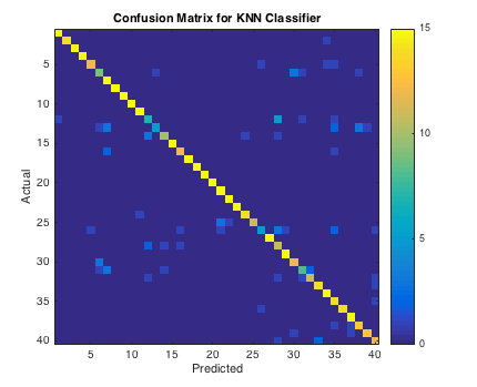
In this confusion matrix for the phoneme classifier, we can see that the vast majority of predictions coincide with the ground truth classification. This is the yellow line along the diagonal. There are a handful of elements which contribute most of the errors.

To correct misclassifications in our program, we implemented a noncausal moving average across the vector of classified phonemes. We considered a window size of 10 for this algorithm, and if we saw that more than 60% of the phonemes in this window were of a certain class, then the phoneme in the middle of that window would be changed to that class. We found that five passes of this algorithm was best in order to get large contiguous regions of a singular phoneme.
In the diagram below, the top row is a sequence of phonemes before the moving average is applied, and the bottom row is the resultant sequence. The extraneous vowels in the string of ‘l’s are removed after the application of the filter.
‘uh’ ‘l’ ‘l’ ‘uh’ ‘l’ ‘l’ ‘oy’ ‘l’ ‘l’ ‘l’ ‘l’ ‘l’ ‘l’
‘uh’ ‘l’ ‘l’ ‘l’ ‘l’ ‘l’ ‘l’ ‘l’ ‘l’ ‘l’ ‘l’ ‘l’ ‘l’

In speech, different speakers take varying times to say identical words. Dynamic Time Warping helped us overcome this problem. DTW is an algorithm that computes a least-cost mapping from timepoints in one discrete-time signal to another discrete-time signal. First, a weight matrix is created for ordered pairs of timepoints in the two signals. Values are only calculated for ordered pairs within a certain distance of the diagonal, because it is assumed that the signals move at similar rates. This is a technique used in research papers on the subject 3. The weight is created by adding the norm of the difference of the two vectors at the given timepoints to the lowest adjacent weight. Once the weight matrix is created, we work backwards from the ordered pair corresponding to the end of both signals. There are three moves that can be made at each iteration: move back in one signal, move back in the other, or move back in both. The move that has the least weight in the weight matrix is chosen. This goes on until the ordered pair (1,1) is arrived at.

Once dynamic time warping has created a map from timepoints in the unaccented speech to timepoints in the accented speech, we can find segments of accented speech that correspond to vowels in the unaccented speech. Then we use our classification model to predict the phonemes that the segments of accented speech are most like. Taking the mode of these classified segments, we find the most viable substitute for the vowel in the unaccented speech. In our project, we were only looking at vowels rather than the whole set of phonemes, because we wanted to downscale our project and believed that most ‘accent’ can be found by looking at the vowels in a speech signal.

So we were able to find the vowel that, in the unaccented speaker’s pronunciation, was the most similar to the vowel spoken by an accented speaker. Because we have samples of the unaccented speech saying all phonemes, we are able to extract sound from those samples and substitute it for the original vowel. The extraction was done by taking overlapping segments of the signal that we wanted to replace the original with, and finding the segment with the highest power, and simply splicing that segment in place of the original vowel. In the place of the original, unaccented vowel, we now have a vowel that is most similar to the way the vowel is spoken in accented speech. We had initially planned to do this by finding a sample of the vowel in the actual speech, but we found that we were not able to make our classification robust enough to get good results in this way.

RESULTS AND FUTURE IMPROVEMENTS:

In our synthesized ‘accented’ speech, we have many substitutions that are either erroneous or too short to make an audible impact. This is primarily due to classification and audio editing errors.

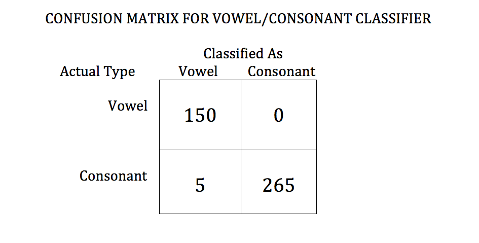
There are numerous improvements we can make, with the most notable one in combining the two classifiers we have in tandem. Considering our vowel classifier classifies the binary ‘is it a vowel or consonant?’ with 98.52% accuracy, and the phoneme classifier identifies every phoneme with a 81.33% accuracy, calculated using leave one out cross validation . If we combined both classifiers it is likely error would have been reduced. Unfortunately, we implemented both of them independent of one another since our original idea was to just use one of them, and rectifying the syntax errors between the two proved to be impractical given our time constraints. Also, using human neural networks instead of KNN could have given us much better results as well. Yet, we felt as if the deep learning mathematics of Neural Networks were far too complex for us to understand, and felt at odds in using a toolbox that quickly computed this for us.

Voice synthesis could also be improved upon. Once the accented version of the phoneme is identified, it is naively pasted into the discrete time spoken signal at the point where energy is highest. More complex methodologies of voice synthesis, such as Google’s WaveNet could be implemented for smoother sounding audio 7.

ADDENDUM:

In our Transformation Folder, ‘english13.mp3’, ‘english19.mp3’,‘english71.mp3’ were the respective British, Southern, and Midwestern accents we wanted to emulate. Two other files, ‘english117.mp3’ and ‘english145.mp3’ were additional files we included that were respectively, a feminine-sounding voice and another British accent. All of these files were from the Speech Accent archive. 8 As illustrated through our transformed audio ‘…_Transform.wav’ and discussed above, we have many short substitutions that do not create a discernible impact to transform the speech. However, notable achievements that resulted in a slight speech transformation occurred at time points throughout our files:
‘english19_Transform.wav’: 0:13 (‘five thick slabs’) 0:26 (‘for the kids’),
‘english117_Transform.wav’: 0:02(‘ask her’) , 0:18(‘a snack’),
‘english145_Transform.wav’: 0:02(‘ask her’), 0:09 (‘six spoons’).
Our file, ‘english117_Transform.wav’, was especially illuminating because of the high prevalence of resubstitution errors. This could be a result of a variety of errors, but we suspect that our training data was not adapted to the variance of pitch this sound file presents. In turn, our classifier results in a great deal of errors, but we could have rectified this situation by including a variety of training data with variable pitch scales.

The confusion matrix for our KNN classifier discussed previously was not appearing due to formatting issues. We have addressed this and it is presented above. The confusion matrix for the vowel/consonant classifier is pictured below. We do not have confusion matrices for the classifier that we do not use because we do not have working code that implements them, since we decided on a KNN Classifier relatively early on in the project.

Works Cited:

http://www.sersc.org/journals/IJSIP/vol5_no1/10.pdf
http://www.dyslexia-reading-well.com/support-files/the-44-phonemes-of-english.pdf
http://www.psb.ugent.be/cbd/papers/gentxwarper/DTWalgorithm.htm
https://www.mathworks.com/matlabcentral/fileexchange/43156-dynamic-time-warping–dtw-
https://www.mathworks.com/matlabcentral/fileexchange/32849-htk-mfcc-matlab/content/mfcc/mfcc.m
https://arxiv.org/abs/1003.4083
https://arxiv.org/pdf/1609.03499.pdf
http://accent.gmu.edu/


Easter Egg? Go to home page and type ‘eecsbit’ Audio on and you’ll hear a mix!

.