November 22, 2016 / by James Connolly / In news

Progress Report 1

Currently, we are still understanding and developing the blocks within our system. Two hurdles beginning our project were MFCC generation and dynamic time warping. Fortunatley, MFCC generation is a well defined problem, and there is well documented,open source code that implements this block in our system. Our worries with MFCCs was that it would not be an effective basis when describing accented phonemes. We found that a naive k-Nearest Neighbors was very effective at classifying accented phonemes using MFCCS, as detailed in our final proposal, proving that MFCCs was a viable basis in which our signal could be represented.

In our project, speakers may take a different duration to speak the same word. This incongruency would result in certain phonemes to be spoken faster or slower than the other, distorting MFCCs. Therefore, we had to implement dynamic time warping (DTW) which addresses this issue by providing a mapping from one signal to another. The struggle with this algorithm was that traditionally it was implemented with the consideration that the input is a 1xN vector. Our inputs, MFCCs, are 13xN matrices, so one difficulty has been adapting the DTW algorithm to allow for this input structure.

Over future plans consist of both finishing and verifying DTW’s implementation (which should be completed by this week). After this, our next challenge will be understanding how effective DTW is at mapping phonemes between each vector in our training set gathered from the Speech Accent Archive. Then, our plan is to generate a dictionary that maps a given phoneme to the same phoneme in a specified accent. Once the dictionary is complete, we will begin system integration, which will consist of designing a script that will take in a spoken calibration signal, a specified accent, and any number of spoken signals to be transformed. The script will output spoken signals transformed such that they have characteristics of the input accent. This script will utilize the DTW, MFCC and the dictionary that we have generated.

One method that we have learned through our research for the project is the Mel-Frequency Cepstrum Coefficient (MFCC). This is a modification of the spectrum of a signal that is a robust way to determine the phoneme that is being voiced. The MFCC is calculated through a series of steps. First the spectrum is calculated through a Fourier transform. Then the logarithm of this spectrum is calculated. Then a small number of overlapping windows are created, usually around 13-19; these are spaced exponentially to mimic the exponential nature of human pitch recognition. The power of the signal within each of these windows is calculated, and the logarithm of the power is taken to mimic the way that the human ear perceives loudness. Thus, a 13-19 element vector with values on the range of 10^1 are obtained. This has a number of benefits for speech processing. For one, it solves the problem of people that speak at different pitches. Since much of speech is harmonic, a traditional spectrum will not pick up similarities between signals that are at different pitches, but the windows incorporated into MFCC calculation account for the minor variations in pitch. Also, the MFCC reduces calculation time, because it has far fewer components than a spectrum, which means that we are working in a much smaller vector space. Finally, the adjustments that are made to account for the way that humans hear, mean that we do not have to do any scaling or weighting after the MFCCs are created.

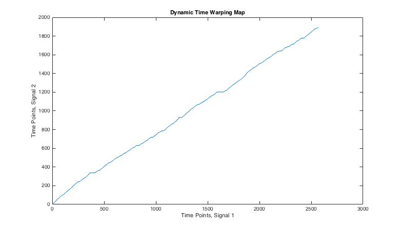
This is a plot showing the map between two speech signals. Each speaker is saying the same sentence, but the number and length of pauses vary, as well as the rate of speech. Therefore, although a linear increasing trend can be seen clearly, there are some variations.

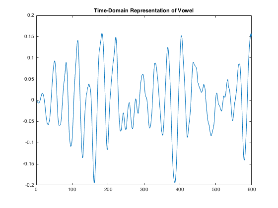
This is a plot of the time-domain representation of a vowel. Although the signal is not perfectly periodic, it is easy to see that it has harmonic content.

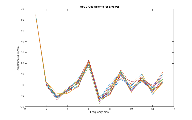
This is a plot of many MFCC vectors calculated from one vowel. Although there are minor variations, there is a clear contour that all of the vectors follow, so they are clustered very closely together in their 13-dimensional vector space.

Authors : Vikram Sacheva, James Connolly, Paul Reggentin